4 Perfect Competition

Perfectly Competitive Market

• price taking
  • a lot of firms on market
  • each firm has small market share
  • no price setting power within individual firm
  • each firm takes market price as given
• product homogeneity
  • perfect substitutions between products
  • no firm can raise price beyond market price realisticly
• free entry and exit
  • no entry or exit costs → suppliers easily enter/exit market
  • buyers can switch between suppliers easily
• FULL INFORMATION
  • no informational asymmetries

Price Elasticity

• Firm has to take market price as given

Profit Maximization

• Profit Function
  • $q$ … Quantity
  • $\pi (q)=R(q)-C(q)$
  • ${\Pi }^{\prime }=0$
  • $MR(q)=MC(q)$
• Marginal Revenue → Marginal Changes
  • $p=MC(q)$
• Second order condition:
  • ${\Pi }^{\prime \prime }<0$ … must be a maximum → otherwise solution does not make sense
  • Profit function must be concave

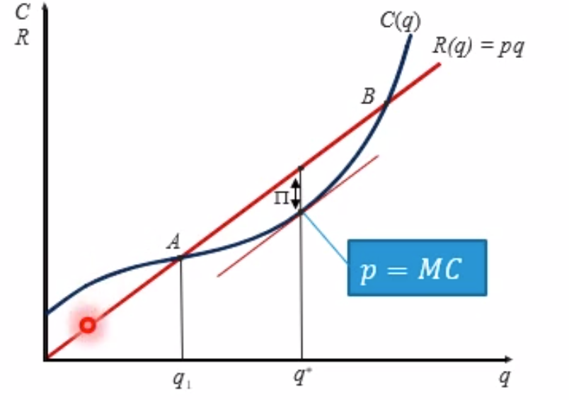
Graphical Solution

• finding largest difference (distance) between revenue function (linear, red) and costs (black, curved)

Demand Curve

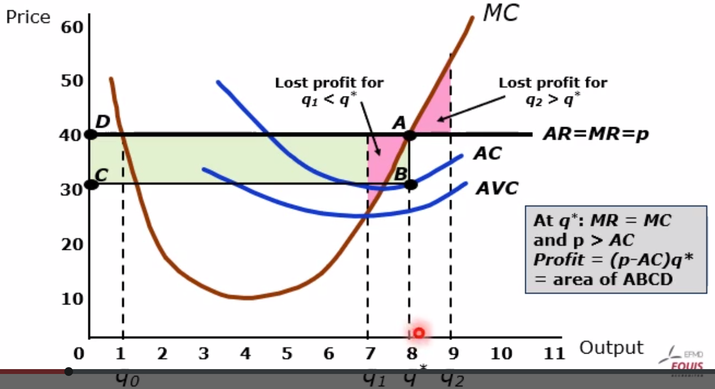
Graphical Solution

• red area → loss of producing more or less than optimal quantity
• have to ensure that producing at the best conditions is better than shutting down
  • saving on fixed costs outweighs the opportunity cost
  • if fixed costs cannot be saved, then operating normally is more beneficial
• 

Shut Down Rules

• if fixed costs are sunk → Past Sunk Cost
  • cannot shut down easily, producing is still better than stopping
• if fixed costs can be recovered / saved → closing is feasibile

Graphical Solution

• own Average Variable Cost must be below industry minimum Average Variable Cost
  • Otherwise there could never be a profit

Industry Supply

• aggregation of all suppliers
  • summing up

Equilibrium

• Equilibrium
  • market clearing price reached → optimal price
  • no excess supply → optimal supply

Long Range Equilibrium

• equilibrium has been reached

• now increase in demand (e.g. change in taste)

• positive profits lead to new players enter the market

• new players means increased supply and lower prices

• lower prices result in zero profits

• equilibrium reached again

• can be run equally for decrease in demand

• profit in the long run is 0

• only supply and demand change, price will not

Competitive Equilibrium

• if costs are … then the long-term supply function is …
  • constant → horizontal
  • increasing → increasing
  • decreasing → decreasing (Economy of Scale)

Short vs Long Term Equilibrium

• short term

  • $P=MC$
  • Average Variable Cost is lower limit of price, otherwise shutting down

• long term

  • $P=MC>AC$ (profitability attracts more firms)
  • supply increases, prices fall, until $P=AC$
  • equilibrium reached → zero profits in long term

Zero Profit Condition

• does not mean that there is no money to be made
• competitive firms are compensated for opportunity costs
• there is no superior investment alternative for them
  • no use selling the business and going after a more lucrative business
• Opportunity Cost is important
  • implicit costs, fictitious employers salary, lost rent revenue

Welfare Characteristics

• 2 parties: Suppliers (Firms) and Consumers
  • Consumer Surplus vs Supplier Surplus
  • what each party gets from the interaction
• Supplier Surplus = Profit
• Pareto Efficiency → maximization of welfare
  • welfare … supplier and consumer surplus
• no definition about distribution of surplus
• one being better off is at the cost of the other
• any Market Failure leads to efficiency loss

Maximum Price

• price ceiling can only be effective if below equilibrium price
  • otherwise still equilibrium price → no effect of policy
• supply is restricted, demand increases
• producers are hurt, since less producer surplus
• Deadweight Loss
  • Total Surplus is less than before
• consumer surplus is greater than supplier surplus
  • if consumer surplus is greater than without policy (at cost of producer surplus) then consumers are effectively better off, otherwise just worse for everyone
  • again: possibility of hurting both suppliers and consumers
• especially with highly inelastic products
  • drugs (additive as well as medical)
  • housing
  • basic food items (potatoes, bread, rice)

Minimum Price

• e.g. minimum wage, essential tax on alcohol, tobacco
• price floor can only be effective if higher than equilibrium price
  • otherwise still equilibrium price → no effect of policy
• demand decreases, supply increases
• suppliers (workers) are hurt, since less suppliers surplus
• overall welfare decreases

Price Support

• government as another consumer → increases demand
• consumer surplus decreases
• producer surplus increases
• overall welfare has increased
  • still a Deadweight Loss since Government pays for more than is gained globally

Production Quota

• maximum quantity to be produced
• companies would like to produce more, but cannot
• consumer surplus decreases
• producer surplus increases
• overall welfare has decreased
• governmental payments for voluntary production restriction
  • larger than overall surplus loss
• Deadweight Loss again

Import Quota

• maximum quantity to be imported into country
  • trade restriction
• results in lower price → market will adjust to price change
• consumers surplus increase
• producer surplus decreases

Import Tariff

• bridge between domestic and world market price
• limiting imports → less imports than without tariffs
• producers will supply more, consumers will demand less
• government will receive tariff amount
• Deadweight Loss (potentially) again

Examples

• Lump-Sum Taxes
  • e.g. taxes on profits
  • ${\Pi }_{net}=(1-t_1)(p\ast q-C(q))$
  • $\frac{\partial \Pi }{\partial q}=(1-t_1)(p-MC(q))=0$
  • $p=MC(q)$
• Taxes on Consumption: Consumption taxes
  • e.g. VAT
  • analogous to decreasing the price, similar to Maximum Price
    • 2 prices, 1 which consumers are paying, 1 which producers are producing with
    • government receives quantity * tax
    • overall loss of welfare → Deadweight Loss
  • ${\Pi }_{net}=(1-t_2)(q-C(q))$
  • $\frac{\partial \Pi }{\partial q}=(1-t_2)(MC(q))=0$
  • $p-t_2=MC(q)$

4 Conditions

• Quantity sold and buyers price, $P_D$ must be on the demand curve
• Quantity sold and sellers price, $P_S$ must be on the supply curve
• $Q_D=Q_S$
• $P_b-P_s=Tax$

Incidence of a Specific Tax

• demand is inelastic → tax burden on consumers
• supply is inelastic → tax burden on suppliers
• Tax burden on consumers in % = $\frac{E_s}{E_s-E_d}$
• Tax burden on consumers in % = $\frac{-E_d}{E_S-E_d}$

Subsidy

• government pays some part of the price
• increases demand
• Deadweight Loss again