5 Monopoly and Monopsony

No more givens

• until now prices were given
• now not anymore

Overview

Buyers / Sellers	One	Few	Many
One	Bilateral monopoly	Limited Monopoly	Monopoly
Few	Limited Monopsony	Bilateral oligopoly	Oligopoly
Many	Monopsony	Oligopsony	Polypoly

Competition vs Monopoly

• competition ⇒ Monopoly
• many sellers buyers ⇒ one seller, many buyers
• homogeneous good ⇒ single product
• free entry for competitors ⇒ limited entry (Market Entry Barriers)
• price is given ⇒ price is set by company (high market power)
• p = MC, p = AC ⇒ profit is maximized by output of $q$ where MR=MC

Market Power

• if players in an Oligopoly are talking to one another they can form an almost monopoly where they can plan their joint supply
  • results in market power similar if not equal to monopoly
• market power … ability to influence the market
  • in perfect competition the price is given → 0 market power

Math and Stuff

Marginal Revenue Function (Linear)

• demand/price: $P(Q)=a-bQ$
• Revenue: $R(Q)=P(Q)\ast Q=(a-bQ)\ast Q=aQ-b{Q}^2$
• $MR(Q)=a-2bQ$
  • same curve, but with twice the slope

Increasing Production

• increasing production will increase the revenue
• but the price needs to be adjusted → demand stays equal
• $MR<p$ … Marginal Revenue always optimal, production below optimum

Price Setting

• in a monopoly there is 1:1 mapping between price and demand
  • we can choose the price and find out about the demand then
• very easy to calculate the revenue
• optimal production rate when factoring in costs
  • Marginal Costs = Marginal Revenue is best production cost
  • $MC=MR$
  • from that we get the optimal quantity to produce
  • from what we can get the price with the demand function

Amoroso-Robinson Formula

$MR=p+p\frac{1}{{\epsilon }_d}$

• ${\epsilon }_d$ … elasticty → Micro Formula Sheet
• in perfect competition: ${\epsilon }_d=-\infty ⟹MR=p$
  • constant marginal revenue: horizontal curves
  • small price increase → complete loss of demand
• market power: $-1>{\epsilon }_d>-\infty ⟹MR<p$
  • negatively sloped market demand & marginal revenue curves
• inelastic demand $-1<{\epsilon }_d<-\infty ⟹MR<0$
  • negative marginal revenue → choose an output level which is in elastic demand

Optimal Prices

$p=mMC$

• $m$ … Markup

Lerner Index

$\frac{p-MC}{p}=-\frac{1}{{\epsilon }_d}$

• Lerner index … left side
• $0<L<1$
• the higher the Lerner index, the less competition
• the higher the markup, the less competition

Industry	Lerner Index	Markup Factor
---
Food	0.26	1.35
Tobacco	0.76	4.17
Textiles	0.21	1.27
Apparel	024	1.32
Paper	0.58	2.38
Chemicals	0.67	3.03
Petroleum	0.59	2.44

Measuring Monopoly Power

• Lerner Index 1 → complete Monopoly
• Lerner Index 0 → perfect competition
• everything in between is some gradual change between extremes

Monopoly and Demand

• more elastic demand → lower markup
• less elastic demand → higher markup

HHI Index

• HHI Herfindahl Hirschmann Index

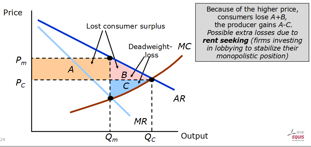
Social Cost

• consumer surplus … difference between willingness to pay and actual price
• producer surplus … profit + fixed costs
• monopoly produces less units at higher price
  • Rent Seeking or Corruption to keep monopoly

Natural Monopoly

• similar to Economy of Scale
• when a single company can produce all the supply cheaper than if the load was split among multiple companies
• very high fixed costs, low variable costs
• subadditive cost function … $f(x,y)<f(x)+f(y)$
  • Baumol
• examples:
  • Railroads
  • Roads
  • Telecommunications
  • Electricity

Regulating the Price

• setting ceiling to the competitive level → not good
  • at this level the company would not work
• setting ceiling such that the company has no profit → perfect
  • company is willing to produce, but has little to no profit
  • best for maximized consumer surplus
  • infeasible due to lobbying and political ambitions

Different Production Costs

• marginal costs should be equal in all sites $M{C}_1=M{C}_2$
• first-order condition still holds:
  • $MC=MR$
• only partial redistribution of production, not complete redistribution

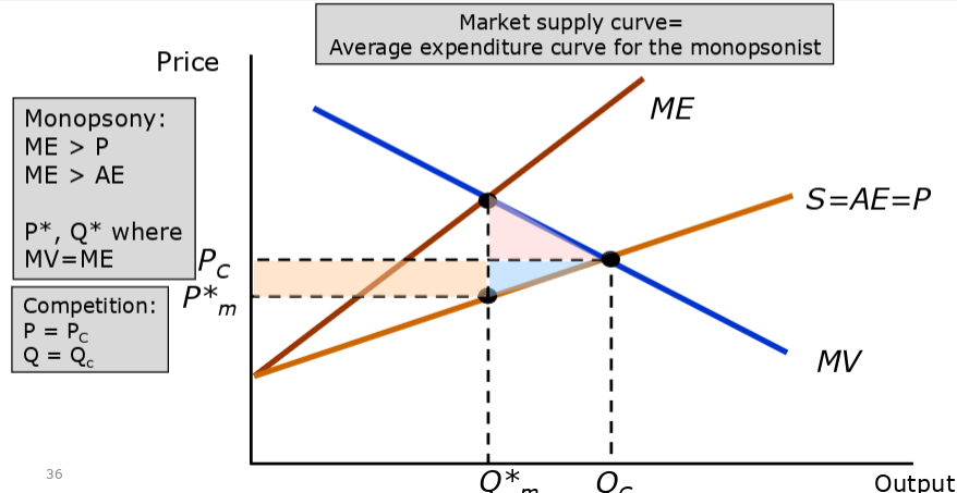
Monopsony

• exact opposite of monopoly
• all market power with demand side
• e.g. military, labor market (in certain industry)
  • military is just 1 per country, but with many defense contractors
  • labor market can force low wages with lower amount of people
• instead of profit there is net value
  • Marginal Value = Marginal Expenditure
• monopsonist buyer wants to maximize net value
• sources of power
  • inelastic market supply
  • small number of buyers (or just 1)
  • little competition between buyers
• Monopoly: Marginal Expenditure = Actual Expenditure = Supply = Value
• Monopsony: Supply = Average Expenditure = Price
  • basically suppliers are forced to produce below market value

Monopoly vs Monopoly

• monopoly
  • MR = MC
  • $q_m<q_c$
  • $p_m>p_c$
• monopsony
  • ME = MV
  • $q_m<q_c$
  • $p_m<p_c$