Consumer Behavior - How Consumers Decide
Consumer Preferences
- assumptions about preferences
- complete → consumer can compare options
- transitivity: A > B and B > C → A > C
- non-satiation: more is better
- if satiation is possible → indifference curve is circular → has an optimum within finite space
- convexity → preference for variety → Monotonicity
- continuity → Marginal Changes
Budget Constraint
- income → cannot spend more than you earn
Consumer Choice
- Utility Function captures preferences
- translating the sloppy terms “nice”, “bad”, etc into numbers → easier to calculate
- Consumer wants to maximize Utility Function under the Budget Constraint
Consumption Bundle
- 2 resources
- each bundle is represented by x and y coordinates of each resource
- some bundles are unobtainable → outside budget constraint
Utility Function
- assigns value “Utility” based on x and y coordinates of a bundle
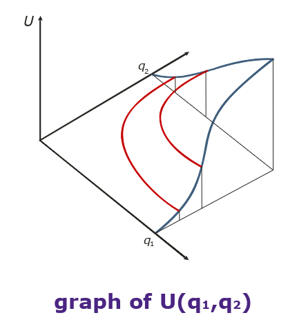
- , … x/y coordinates of bundle
- … Utility of bundle
Indifference Curves
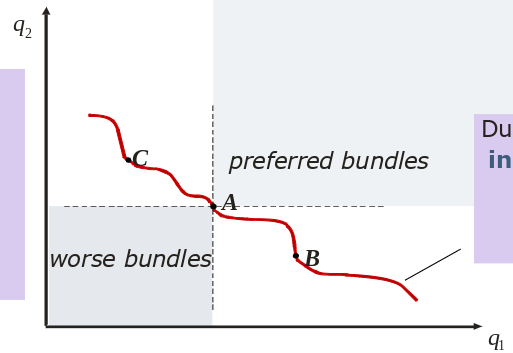
- bundles which are “equal” → same utility
- preferred bundles → more of or or both increases utility → farther from origin
- worse bundles → less of or or both decreases utility → closer to origin
- no indifference curves intersect → transitivity
Convexity
- preference of variety
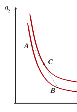
- combining A and B to produce optimal point C
- Concavity → mixture of A and B would result in a lower utility than A or B → against convexity principle
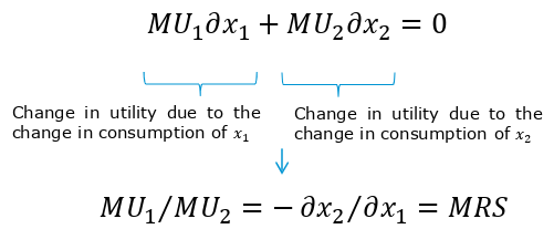
- slope of indifference curve is the relative value of the good → Marginal Changes
- called here; Marginal Rate of Substitution
Marginal Utility
Curvature of Indifference Curves
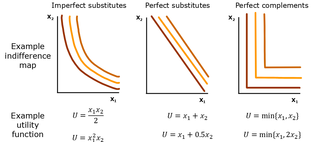
- substitutes → one can substitute the other
- complements → one cannot substitute the other
- perfect, could not be more extreme
Why does this cost money tho?
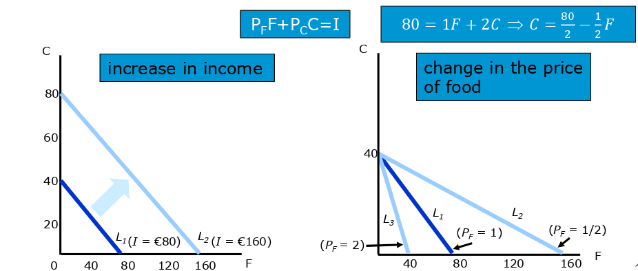
Budget Constraint
- Income limits the possible bundles
- changes in income shift the limit outwards/inwards
- changing the prices is about moving the intersect of that axis
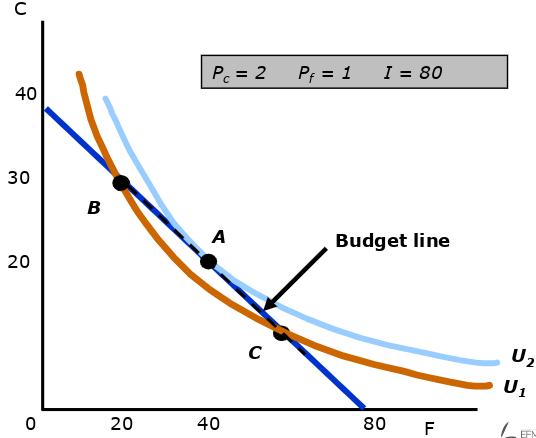
Indifference Curve and Utility
- taking any indifference curve and finding the 2 intersections of the budget constraint
- the region between indifference and budget curve yield higher utility and are obtainable
- drawing another function through one point within this region
- repeat finding the intersects
- repeat drawing a curve through region between 2 curves
- after iterations one will reach a tangent point which has maximized the utility
Slopes at Points
- C: slope of utility function > slope of budget line → move to left
- B: slope of utility function < slope of budget line → move to right
- A: slope of utility function = slope of budget line → stay where you are
Boundary Solutions
- highest utility is at one of the boundaries
- absolute dominance of one product over the other

Playing with the numbers
- higher price → less quantity
- at each price map the distribution of products
- purple line left: continuous price-consumption curve → how the consumption changes when costs increase/decrease
- purple line right: continuous income-consumption curve → how the consumption changes when the overall income changes
- demand curve: capturing preference of individual, not specific actions
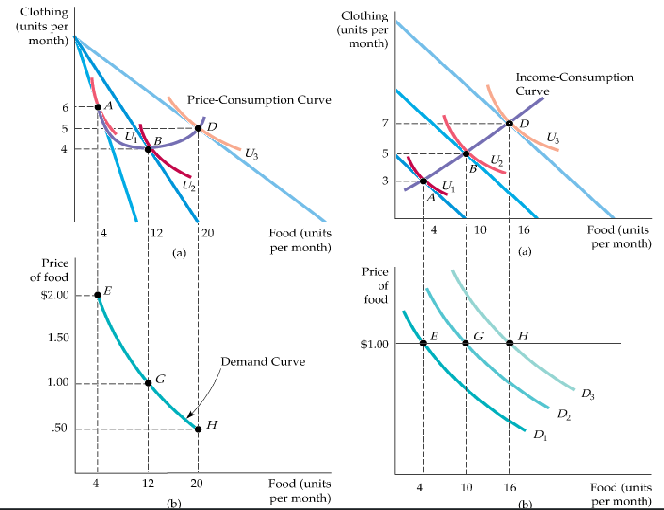
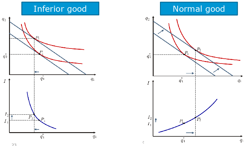
Engel Curve
- Demand by Income
- again, just preferences of individual
- slope and monotonicity of Engel curve (lower respectivel) is important
- rising → normal good (cars)
- falling → inferior good (hand-made brooms)
- non → quasilinear → demand does not change when income changes
Deriving Individual demand function
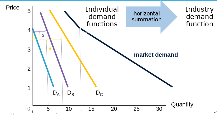
Sum it all Up → Market Demand
- each individual has different preferences
- summing up all individual preferences creates demand
- horizontal summation
- 0 + 5 + 8 = 13
Substitution and Income Effects
- Substitution Effect → changes in market demand regarding relative price changes
- Income Effect → changes in market demand regarding non-relative price changes (or income changes)
- Substitution Effect → changing the price relatively → demand will increase/decrease
- Income Effect → changing the price absolutely → income changes relatively → demand will increase/decrease