Homework FMa 2

Merged Markdown Document

Task 1: Who is part of the “labor force” and which people are “out of the labor force”?

The “labor force” constitutes two parts of the population:

• Unemployed: Those who are actively seeking employment.
• Employed: Those who have jobs.

The “out of labor force” consists of those people who are of working age (15-64) but are not actively seeking employment for various reasons (e.g., students, pensioners, homemakers, etc.).

Task 2: How are the employment rate and the unemployment rate defined?

The employment rate is defined as the percentage of the labor force who have a job.

$\text{Employment Rate}=\frac{\text{Employed}}{\text{Labor Force}}\ast 100$

Similarly, the unemployment rate is defined as a percentage of the labor force who do not have jobs but are actively seeking work.

$\text{Unemployment Rate}=\frac{\text{Unemployed}}{\text{Labor Force}}\ast 100$

Task 3: Explain the concept of the reservation wage.

The reservation wage is the minimum wage level at which a worker is willing to accept a job, influenced by alternative opportunities such as unemployment benefits. It varies among individuals based on factors such as how much one can buy with unemployment benefits or how much one values free time, experience, and personal financial situations. Essentially, it represents the lowest acceptable compensation for their labor. The reservation wage also accounts for the opportunity cost of remaining unemployed, playing a crucial role in labor supply dynamics, as it determines whether potential workers will consider a job or remain unemployed based on the offered wages relative to their expectations and alternatives.

Task 4: Explain the concept of efficiency wages. Why would employers pay higher wages?

Efficiency wages are wages that employers choose to pay above the market equilibrium level, motivated by several factors that benefit the organization. By offering higher wages, employers can increase worker productivity, reduce turnover rates, attract higher-quality candidates, and foster loyalty among employees. When workers perceive their pay as competitive and fair, they are more likely to be motivated, committed, and invested in their work, ultimately leading to significant cost savings in recruitment and training while enhancing overall business efficiency.

Task 5: On which factors does the bargaining power of the workers depend?

The bargaining power of workers depends on the following factors:

1. The nature of the job and cost to replace the worker: Individual workers with unique or rare skills, better education, or longer/varied work experience have a higher bargaining power than less educated persons or those with more general skills.

2. Labor market conditions: The bargaining power of workers correlates positively with the probability that a worker can find an alternative job. It typically increases during periods of economic growth and lower unemployment rates, and decreases during crises. It is also generally lower in less competitive industries characterized by monopsonic employers.

3. Labor rights determined by the legal and institutional framework: Employee protection such as minimum wage, strong labor unions, and higher unemployment benefits increases the collective bargaining power of workers.

The mentioned factors affect labour supply and/or demand: when supply is lower, and industry demand is higher, the bargaining power of workers increases, or vice versa. The bargaining power of workers, in turn, affects the amount of wage they are willing to accept (reservation wages).

Task 6: What is the value of the price premium $m$ in a market with perfect competition?

The price premium $m$ is defined as the markup of the price over the marginal cost that businesses can charge due to possessing some market power as a result of imperfect competition.

In a market with perfect competition, firms do not have market power due to the large number of buyers and sellers with complete knowledge of the market, and free exit and entry of firms selling a homogeneous good.

This results in firms being ‘price takers’, meaning they must accept the equilibrium price where $P=MC$ at which goods are sold in the market. If a perfectly competitive firm attempts to charge even a tiny amount more than the market price, it will be unable to make any sales, indicating the value of $m$ is zero.

Task 7: What is the relationship between the natural rate of unemployment and the natural level of production?

The natural rate of unemployment is the unemployment rate at which the actual price level is equal to the expected price level. For a given labor force, the natural unemployment rate determines the level of employment, and given the production function, the level of employment determines the level of output.

Expressed mathematically, when the unemployment rate is equal to the natural rate $u_n$, employment is given by $N_n=L\times (1-u_n)$ and the output is equal to:

$Y_n=A\times N_n=A\times L\times (1-u_n)$

(where $N_n$ is the natural level of employment, $A$ is labor productivity and $Y_n$ is the natural level of production). Consequently, a lower natural rate of unemployment is associated with a higher natural level of production $Y_n$, and vice versa.

It makes logical sense as well: a lower natural unemployment rate implies that more workers are employed in productive activities, boosting economic output. The natural level of production grows when more workers are employed, assuming labor productivity remains constant.

Task 8: Present the wage-setting curve verbally and graphically.

The wage-setting equation is given by:

$\frac{W}{P}=F(u_{+},z_{-})$

where:

• $W$ is the nominal wage,
• $P$ is the price level,
• $u_{+}$ is the unemployment rate, and
• $z_{-}$ represents other factors that may affect wage setting (such as unemployment benefits).

The price level, $P^e$ , affects nominal wages because employers and employees care about real wages, not nominal. Real wages deal with the purchasing power, simply, the two parties care about how much money they can pay or receive, relative to the goods that they sell or buy. For instance, if workers expect the prices of the goods that they buy to double, they will demand double the amount of their nominal wages to maintain their real income. The same logic applies to employers; they would be willing to double the nominal wages. Wage-setting reflects economic conditions, hence why they concern price levels.

The unemployment rate, u, has an indirect relationship with real wages; as u↑, nominal wages decrease, vice versa. When the rate of unemployment is low, this gives workers a higher bargaining power than employers, as they can easily replace the job with another and can obtain higher wages. Conversely, when the rate is high, this gives workers a lower bargaining power because the firms can easily replace them with others whereas it will be hard for the workers to find another job. Additionally, this variable causes a movement along the WS curve.

The catch-all variable, z, has a direct relationship with wages; as z↑, nominal wages increase. This too can be illustrated below with $\frac{W}{P}=F(u,z)$ where:

• $PS$ = the price-setting relation,
• $WS$ = the wage-setting relation, and
• $A$ = the natural rate of unemployment ($U_n$).

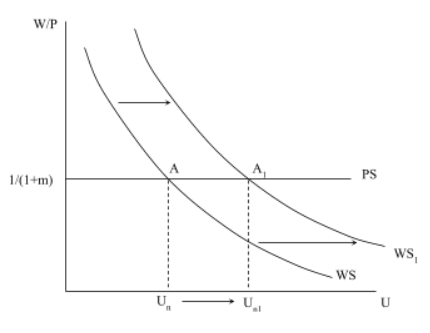
When $z$ increases (increase in unemployment benefits), this leads to a rightward shift from $WS$ to $W{S}_1$ as workers demand higher real wages, $W/P$. Consequently, this sets the new equilibrium, $A$ , and an increase in the natural rate of unemployment $U_1\to U_{n-1}$ . $z$ is the only variable that can cause shifts of the WS curve.

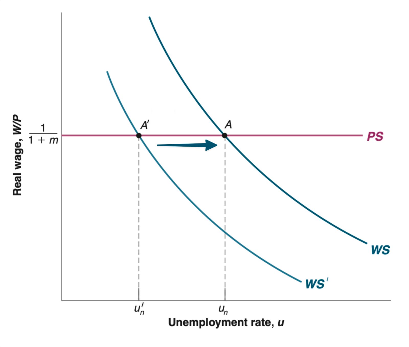
Task 9: Assume that unemployment benefits decrease. Analyze this change verbally and graphically.

A decrease in unemployment benefits, represented by a decrease in $z$, affects the labor market as follows:

• Downward Shift of the Wage-Setting Curve: Lower unemployment benefits reduce workers’ bargaining power, leading to a decrease in the real wage for any given unemployment rate. This shifts the wage-setting curve (WS) downwards.
• Movement Along the Price-Setting Curve: The price-setting curve (PS) remains unchanged as it is determined by firms’ markup decisions.
• New Equilibrium with Lower Unemployment: The new equilibrium point occurs at a lower real wage and a lower unemployment rate. The reduced bargaining power of workers leads them to accept lower real wages, allowing firms to hire more workers.

10. Derive the original Phillips curve from the wage and price setting equations. How is expected inflation formed? Explain how the actual inflation is related to ${\pi }^e$, $m$ and $u$.

The original Phillips curve can be derived from the wage and price setting equations, highlighting the relationship between inflation, expected inflation, and unemployment.

• Wage Setting Equation: The nominal wage ($W$) set by wage setters depends on the expected price level ($P^e$), the unemployment rate ($u$), and other factors ($z$) that affect wage determination:

• $W=P^{e}F(u,z)$

  • For simplicity, we assume a specific form for the function F(u, z): $F(u,z)=1-\alpha u+z$ where α captures the effect of unemployment on wages.
  • Substituting this form into the wage setting equation, we get: $W=P^e(1-\alpha u+z)$

• Price Setting Equation: The price level (P) set by firms depends on the nominal wage (W) and the markup (m):

• $P=(1+m)W$

• Combining the Equations: Substituting the nominal wage from the wage setting equation into the price setting equation, we get a relationship between the price level, the expected price level, and the unemployment rate:

• $P=P^e(1+m)(1-\alpha u+z)$

• Expressing in Terms of Inflation: This equation can be rewritten in terms of inflation ($\pi$) and expected inflation (${\pi }^e$):

• $\pi ={\pi }^e+(m+z)-\alpha u$

  • This equation shows that actual inflation is influenced by expected inflation, the markup, other factors affecting wage determination, and the unemployment rate.

Detailed Derivation of the Phillips Curve

$P=P^e(1+m)(1-\alpha u+z)$ We now use time subscripts for the price level (P_t), the expected price level (Pe_t), and the unemployment rate (u_t) to indicate their values in year $t$, which modifies the above Equation accordingly. $P_t=P_t^e(1+m)(1-{\alpha }_{t+z})$

Next, we transition the expression from price levels to inflation rates by dividing both sides of the equation by last year’s price level, $P_{t-1}$. $\frac{P_t}{P_{t-1}}=\frac{P_t^e}{P_{t-1}}(1+m)(1-{\alpha }_t+z)$

Rewriting the fraction $\frac{P_t}{P_{t-1}}$ as: $\frac{P_t}{P_{t-1}}=\frac{P_t-P_{t-1}+P_{t-1}}{P_{t-1}}=1+\frac{P_t-P_{t-1}}{P_{t-1}}=1+{\pi }_t$. Here its important to remember the inflation rate ${\pi }_t\equiv \frac{P_t-P_{t-1}}{P_{t-1}}$

Now lets do the same for $\frac{P_t^e}{P_{t-1}}$ with ${\pi }_t^e\equiv \frac{P_t-P_{t-1}}{P_{t-1}}$: $\frac{P_t^e}{P_{t-1}}=\frac{P_t^e-P_{t-1}+P_{t-1}}{P_{t-1}}=1+\frac{P_t^e-P_{t-1}}{P_{t-1}}=1+{\pi }_t^e$

Now let’s replace $\frac{P_t}{P_{t-1}}$ and $\frac{P_t^e}{P_{t-1}}$ in the Equation we got to after the time modification we get: $(1+{\pi }_t)=(1+{\pi }_t^e)(1+m)(1-{\alpha }_{t+z})$ This results in a relationship between inflation ($p_t$), expected inflation ($p{e}_t$), and the unemployment rate ($u_t$), with subsequent steps refining this relation to appear more user-friendly.

Now we divide both sides by $(1+\pi t^e)(1+m)$: $\frac{(1+{\pi }_t)}{(1+{\pi }_t^e)(1+m)}=1-\alpha u_t+z$

As long as inflation, expected inflation, and the markup remain reasonably small, a satisfactory approximation for the left side of the equation is $1+{\pi }_t-p_t^e-m$. Substituting this into the previous equation and rearranging yields:

${\pi }_t={\pi }_t^e+(m+z)-\alpha u_t$

Removing the time indexes, this can be referred to as the original Philips curve. Including the time indexes (${\pi }_t^e=\bar{\pi }$) simplifies it as well. The inflation rate, represented as ${\pi }_t$, is influenced by the expected inflation rate, denoted as ${\pi }_t^e$, and the unemployment rate, $u_t$. Additionally, this relationship is contingent on the markup, $m$, factors influencing wage setting, $z$, and the impact of the unemployment rate on wages, $a$.

${\pi }_t=\bar{\pi }+(m+z)-\alpha u_t$

Expected Inflation Formation

Expected inflation formation depends on how anchored expectations are.

• Anchored Expectations: If inflation is stable (relatively constant over time)and not persistent (with a increasing or decreasing trend), wage setters might expect this year’s inflation to be similar to a long-term average ($\bar{\pi }$):
• ${\pi }_t^e=\bar{\pi }$
  • This was the case in the period studied by Phillips, Samuelson, and Solow, leading to the original Phillips curve.
• De-anchored Expectations: If inflation becomes more persistent, wage setters might base their expectations on past inflation:
• ${\pi }_t^e=(1-\theta )\bar{\pi }+\theta {\pi }_{t-1}$
  • Here, θ captures how much weight is given to last year’s inflation (${\pi }^e$).
  • When $\theta$ equals zero, we get the original Phillips curve, a relation between the inflation rate and the unemployment rate

Relating Actual Inflation to Expected Inflation, Markup, and Unemployment

• Equation: The relationship between actual inflation ($\pi$), expected inflation (${\pi }^e$), markup ($m$), and unemployment ($u$) is given by:
• $\pi ={\pi }^e+(m+z)-\alpha u$
• Explanation:
  • Expected Inflation (${\pi }^e$): An increase in expected inflation leads to higher wage demands, pushing up prices and actual inflation.
  • Markup ($m$): A higher markup increases prices directly, leading to higher inflation.
  • Unemployment ($u$): Lower unemployment means a tighter labor market, leading to higher wages and prices, thus increasing inflation.
  • Other Factors ($z$): Any factors that increase wage demands (e.g., more generous unemployment benefits) will also lead to higher inflation. This equation summarizes the key dynamics of the Phillips curve, illustrating how these factors interact to determine the level of inflation in the economy.

Task 11: What relationship does the modified Phillips curve represent?

The modified Phillips curve shows the relationship between inflation, expected inflation, and unemployment. It represents the negative relationship between the unemployment rate and the change in the inflation rate, indicating that lower unemployment rates generally correspond to higher inflation rates.

The modified Phillips Curve is expressed as:

${\pi }_t={\pi }^e+(m-z)-\alpha u_t$

where:

• ${\pi }_t$ is the current inflation rate,
• ${\pi }^e$ is the expected inflation rate,
• $m$ is the markup,
• $z$ is other factors affecting wages, and
• $\alpha$ is the sensitivity of inflation with respect to unemployment.

Expected Inflation Rate

The expected inflation rate is dependent on how people form their expectations about inflation. It can be formed by either of these two scenarios:

1. If people’s expectations of inflation are anchored ($\theta =0$), we return to the original Phillips curve: ${\pi }_t=\pi +(m-z)-\alpha u_t$
2. If the current year’s inflation rate completely depends on the previous year’s ($\theta =1$), the function adjusts accordingly. ${\pi }_t=\pi +(m-z)-\alpha u_t⟹{\pi }_t-{\pi }_{t-1}=(m-z)-\alpha u$