Homework GT1 Experiments 8 to 11

by Matthaeus Engelbrecht (12318768), Elias Prackwieser (12300748), Benjamin Meixner (12302260)

Experiment 8 - Dictator Game

a) Is this a Game?

for it to be considered as a Game in Game Theory, it needs to fulfill the following 3 criteria: (i) Players with (ii) potential strategies that have certain (iii) utility payoffs associated with combinations of strategies. This game has two players, with payoffs, but not potential strategies, as only Person A is able to act in this game. Person B is only able to receive something. Therefore it is not a game.

b) Optimal Strategy of A

The optimal strategy of Person A is, to offer B the lowest possible amount of money. This is because Person A has to assume full rationality of Person B. In this context this means that Person B will accept any amount, even if they see it as “unfair”, as the other option would be to get nothing. This is therefore an empty threat, and nothing for person A to worry about. To recap, the optimal strategy for Person A is to offer Person B E$ 0.10.

c) Actual Data

The data represents the theory wonderfully. The mode is 99.9 for Person A/0.10 for Person B. This happened a total of 17 out of 31 times. Another 8 Player A’s played, what 9 would call an almost optimal strategy, and gave player B everything between 0.11 and 10. I think these also saw the optimal strategy, but didn’t want to push their luck too much. A total of three Players played it “fifty-fifty”. I would guess these did it either out of empathy, or a misunderstanding of the assignment. Two players gave away all of their money. These very probably didn’t understand the assignment, or felt extra generous that day.

When looking at the data, what is most surprising to me, is that not a single Player B rejected the offer. This underlines that player B, even if they might be unhappy with their price, will act rationally.

In conclusion most players played the optimal strategy and empty threats don’t work.

2. Experiment 9 - Ultimatum Game

a)

sequential

b)

possible strategies player A:

• the possibilities are almost arbitrary with 1 cent jumps resulting in 10$ * 100 cents - 10 cents minimum = 1990 possibilities
• we reduce the options to 4 to reason better and derive insights easier, since they should be valid with wider sets

A1: offer 0.10 A2: offer 25 A3: offer 50 A4: offer 75

possible strategies player B:

2^4 = 16 Strategies

1. Reject all offers: (= 0.10 → R, >= 25 → R, >= 50 → R, >= 75 → R)
2. Accept 0.10, reject the others: (A, R, R, R)
3. Accept 25, reject the others: (R, A, R, R)
4. Accept 50, reject the others: (R, R, A, R)
5. Accept 75, reject the others: (R, R, R, A)
6. Accept 0.10 and 25, reject the others: (A, A, R, R)
7. Accept 0.10 and 50, reject the others: (A, R, A, R)
8. Accept 0.10 and 75, reject the others: (A, R, R, A)
9. Accept 25 and 50, reject the others: (R, A, A, R)
10. Accept 25 and 75, reject the others: (R, A, R, A)
11. Accept 50 and 75, reject the others: (R, R, A, A)
12. Accept 0.10, 25, and 75, reject the others: (A, A, R, A)
13. Accept 0.10, 50, and 75, reject the others: (A, R, A, A)
14. Accept 25, 50, and 75, reject the others: (R, A, A, A)
15. Accept all offers: (A, A, A, A)

BUT we can reduce it by setting a minimum for B and accepting any offer of A which is greater or equal to the minimum B will tolerate since anything above the threshold is “extra utility” from the perspective of B

Offers of A: (0.10, 25, 50, 75)

1. Accept = 0.10: (A, A, A, A)
2. Accept >= 25: (R, A, A, A)
3. Accept >= 50: (R, R, A, A)
4. Accept >= 75: (R, R, R, A)

solving for Nash Equilibria:

Offer of A	= 0.10	>= 25	>= 50	>= 75
0.10	A	R	A	R
0.10	A	R	R	A
0.10	A	A	A	R
0.10	A	A	R	A
0.10	A	R	A	A
0.10	A	A	A	A
25	R	A	R	R
25	R	A	A	R
25	R	A	R	A
25	A	A	R	R
25	R	A	A	A
25	A	A	A	R
25	A	A	R	A
25	A	A	A	A

similarly for A3 = 50 and A4 = 75

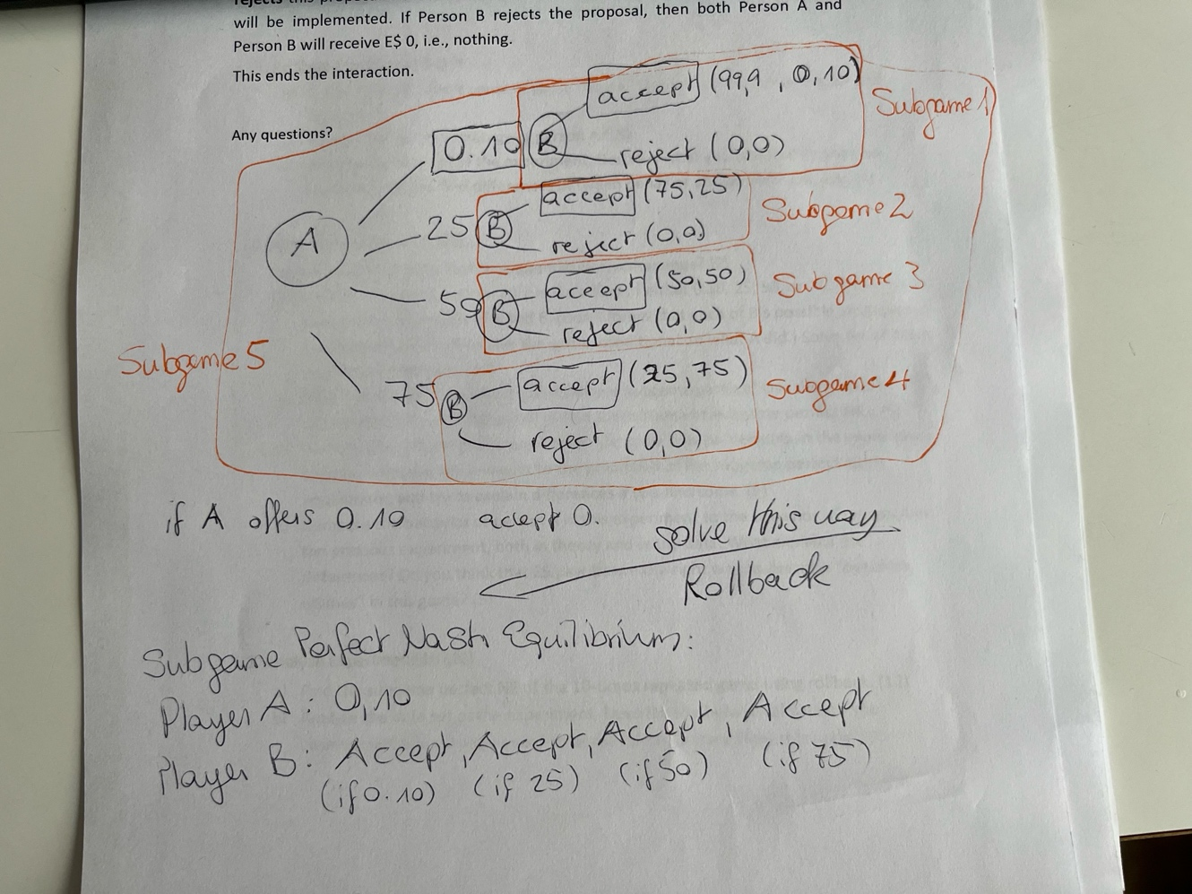
c)

Finding SPNE at (0.10; A, A, A, A) with extensive form

• accepting for B is always the better option than rejecting
• therefore best strategy of A is to offer least i.e. 0.10$

d) Data Set

• only two players A followed the perfect strategy – the rest made “irrational” offers (the average offer to players B is 40,2 !!!)
• players A seem particularly keen on making a “ok - fair” offer to player B because they fear that player B might reject their (not so fair) offer …
  • … however if player B would be perfectly rational there would be no reason to not accept player A’s offer in this **one shot ultimatum game (**0.10 > 0) …
• players A might also just enjoy the “safety” of offering A a deal they cannot refuse to get a higher yield from the transaction as soon as we might expect B to be a little crazy
• nonetheless, 8 out of 32 players B rejected the offers

reasons: fear, irrationality, defiance, psychology (!) → you want to harm the “outgroup” to earn a better image of yourself …

e) Differences in behavior of person A

in Theory:

• no difference in behavior if we assume rationality of player B in Data:
• great differences → player A might fear player B’s irrationality/human behavior … “fairness”

E$ payoffs are not an optimal way to describe outcome utilities in this game. Why? Because money represented in numbers in some foreign currency is something very abstract. It would be interesting to see how the results of the experiment would change if something more tangible e.g. apples would be used as “outcome utilities”

3. Experiment 10: Repeated Ultimatum Game

• Repeated Ultimatum Game

a)

finding SPNE using rollback by finding the best action for every possible point/subgame along the sequence

Round 10: (person A offers 0.01$; person B accepts)

• person B acts rationally and accepts any offer greater than 0$\dots personAknowsthisandwilltrytomaximizehisprofitaccordingly->offering0.10$ to person B

same explanation for the other rounds:

Round	Best Offer A	Reaction B
9	0.01	accept
8	0.01	accept
7	0.01	accept
6	0.01	accept
5	0.01	accept
4	0.01	accept
3	0.01	accept
2	0.01	accept
1	0.01	accept

b)

Observations:

• more cooperative atmosphere at the end
• learning from past experiences (reputation)
• convergence to “fairness” till round 6 → then, person B is receiving lower offers again
  • till the end B has weaker reputation-based threats
  • last round there is no basis for deviating from 0.10$ → threat empty

→ average payoff for player A in each round:

• we see a rise in profitability over 10 rounds:
  • but we can also see that B collectively always receives less than A

Experiment 11 - Market Game

• Market Game

a) Type of Game

This is a simultaneous Game, as Players A and B act first with C following them

b) Find all subgame perfect Nash equilibria of the single round game. (10)

To find the Nash equilibrium, we need to start with Player C’s optimal strategy: $\text{Offer A}>\text{Offer B}\to \text{pick offer A}$ $\text{Offer A}<\text{Offer B}\to \text{pick offer B}$ $\text{Offer A}=\text{Offer B}\to \text{pick either offer}$ As both Player A and B are rational, they both know Player C’s strategy. Therefore, they will try to undercut each other until the maximum offer (for Player C), 8$ is reached. The best response for Player A and B is to offer 8$. 8$/8$ is the subgame perfect Nash equilibrium.

c) Analyzing the Data

The average offer changed drastically over time.

Round	Avg Offer A_A	Avg Offer A_C	Avg Offer B_B	Avg Offer B_C	Avg offer	Profit A	Profit B	Profit C	Max offer X_C	Min offer X_C
1	4,08	5,92	4,60	5,40	4,34	1,73	1,80	6,46	8	3
2	3,41	6,59	3,64	6,36	3,53	1,89	0,87	7,24	8	3,5
3	3,05	6,95	3,65	6,35	3,35	1,21	1,45	7,34	8	0,01
4	3,21	6,79	2,89	7,11	3,05	1,30	0,93	7,30	8	4
5	2,57	7,43	2,66	7,34	2,61	1,42	0,82	7,75	8	4

In the first round the average offer from Player A and B was 4.34, which was still a somewhat “fair” split, but by the last round this offer almost halved to 2.61. This shows how the rejection by Player C taught A and B into lowering their own share. Player C was steadily doing better each round.

This data also shows the difference between the average offer (for Player A and B’s own share) and the average profit for Player A and B beautifully. On Average the accepted offer was 40% of the proposed offer. This stayed steady throughout the rounds (Round 1-5: 41%, 39%, 40%, 36%, 43%).

d) Differences between Nash Equilibrium and the Data

In theory, both Player A and B would offer both 8/$. In Our data we have a few differences. In our previous experiments with multiple rounds, we oftentimes had a quick approach to the optimal strategy. Here however, it is (on average) never reached. The approach is still there, though.

I think, this is for two main reasons. (1) The players switched their Role often, (1.1) so some might’ve been in the same position for a long time and (1.2) didn’t have enough rounds to converge to the Nash equilibrium. (2) Players A and B were hoping to collude in a way, as they saw how others didn’t offer the maximum amount to Player C. In comparison, in our previous games the equilibrium was reached pretty fast by one, and then subsequently all players.